The Origin of Mass

The Origin of Mass

The inertial mass of matter is caused by the fact that any extended object must necessarily exhibit inertial behaviour

... even if its constituents themselves do not have any rest mass. This is a consequence of the finite speed of light at which the binding forces propagate between those constituents.

1. Summary

The origin of mass is one of the central unresolved questions in modern physics. For quite a long time physicists have been looking for a reason why matter should display inertial behaviour. The search for the Higgs boson is one example of this. However, the Higgs model is not the answer to this question, as will be shown.

There is a simple and very fundamental way to explain inertial mass. If two objects are bound to each other such that the binding field enforces a specific separation, then each time the position of one of them changes, a finite time elapses before the other particle moves, due to the finite speed of light. This delay is sufficient to explain inertial behaviour.

From the above argument, it turns out that the inertial mass of an elementary particle is given by the universal equation

where R is the radius of the particle. The validity of this equation can easily be checked for elementary particles carrying an electric charge. In such cases, the radius R follows classically from the magnetic moment, and when this radius is inserted into the above equation it yields the correct mass!

This explanation of mass requires a model of an elementary particle in which it is composed of 2 sub-particles. Although such a model conflicts with currently accepted theoretical physics, it does not contradict any experimental observations, provided the model presented here is applied consistently.

Furthermore, the relativistic increase in mass due to motion and the resulting mass-energy formula (Einstein) are explained perfectly by this mechanism.

The origin of mass is therefore no longer a mystery in physics.

(Note: This site is also available as a pdf file)

2. A Physical Model of Inertial Mass

When a physical object has an extension, there can be two possible reasons:

The planetary case: The constituents each have a mass and orbit each other. The centrifugal inertial force balances the attractive force. Examples of this include the planetary orbits of the solar system and the Bohr model of the atom
The multipole case: The constituents are bound together while at the same time being kept apart by a multipole field originating in each of the constituents. A classical example of this is the individual atoms that make up a molecule.

Only the second alternative can be used in the case considered here, since we wish to explain the existence of mass in a configuration in which the basic constituents have no mass.

We will therefore investigate the situation of two fundamental ("basic") particles, which have no mass and which are bound to each other at a separation r₀ . Such a bond at a distance is, as we have explained, realised by a multipole field, meaning that one particle (B) resides at the minimum of the potential of the field due to other particle (A) and vice versa, as shown in the figure 2.1. In each case, U is the binding potential.

Figure 2.1:

The field of particles A and B bound to each other to maintain a separation r₀

If one of the particles, e.g. particle A, is now held in a fixed position and the other, particle B, is moved towards or away from particle A by a certain amount Δr, the field tries to move particle B back to its original separation r₀ from A. Hence a force must be applied to achieve this displacement.

Now consider a different situation. If neither of the particles is fixed and one particle, e.g. B, is moved by an external force, the other particle will follow. However, this will not happen instantaneously. The change in the field caused by the change in position of particle B can only propagate at the speed of light c. This means that for a time interval given by

(2.1)

particle A is still held in its position by the “old” field of particle B, which has not yet changed. Also, the field due to particle A is unchanged at the position of particle B and therefore tries to keep particle B in its place. This means that a force is necessary to move particle B.

After a time Δt, the change in the field due to particle B will reach particle A, which will now move with the field to a position that corresponds to the new position of particle B. Consequently, after a further period of time Δt the field due to particle A at the position of particle B will adjust to the new position of particle A, and the force acting on the displaced particle B will disappear. Now both particles will be moving and no force will be necessary any longer.

A detailed step-by-step illustration of this process may be found here.

Top

3. Quantitative Determination of the Mass of an Elementary Particle

To calculate this effect quantitatively, it is necessary to know the structure of the field binding the two particles.

To determine the structure of this field we will use the approach that the binding field between the two particles should be the simplest type of multipole field. It corresponds to that shown in the above diagram (figure 2.1):

(3.1)

where F is the force due to the field, S is the field constant, which associated with the strong force; r is the distance between the two particles in the multipole configuration, and r₀ the equilibrium distance (corresponding to Δr=0) at which the force disappears.

In the following we will only consider small accelerations, where ‘small’ means that during a time Δt the acceleration leads to a change in velocity, Δv << c. For such changes, the denominator of (3.1) can be assumed to be constant over the time interval Δt.

We will now consider the case where the particle B is accelerated at a constant rate starting at a specific moment.

Then for a time

(3.2)

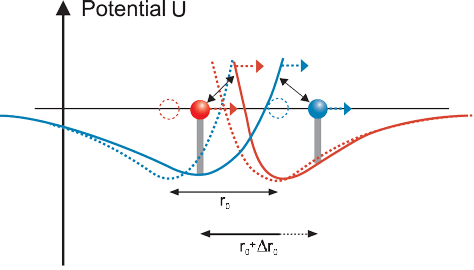
after the onset of the acceleration, the field at particle A will not have any information about this change in position – due to the finite speed of light c – and will therefore remain as it is. Immediately after this initial period, Δt₁, particle A will then be accelerated constantly. The acceleration of particle A will follow the acceleration of particle B with this time delay Δt₁. On the other hand, the change in the field caused by the changing position of particle A will reach particle B after a further delay of Δt₁. This delay leads to a constant, additional displacement of the fields between the particles, resulting in a constant force between them. - This situation is portrayed in figure 2.2.

Figure 3.1:

Configuration of the field at constant acceleration -
The dotted objects show the parts and fields at rest, the solid objects and lines the situation after the right particle has been set in motion

Assuming that a constant acceleration a acts on B, particle B will have moved a distance

(3.3)

during the time 2Δt₁, which is now added to the equilibrium distance. According to eq. (3.1) the retarding force on particle B in the direction of motion, F_dm, will increase to the value

(3.4)

where Δr is given by eq. (3.3).

So particle B will experience a constant force given by

(3.5)

or, using (3.2) (i.e. Δt₁ = r/c) for the time offset,

(3.6)

According to Newton’s definition, inertial mass is given by

Top

and therefore

(3.7)

Returning to eq. (3.4), we must now remember that the full force

is only effective if both basic particles are positioned on a line parallel to the direction of the applied force.

Due to their orbital motion, the basic particles are in fact positioned at varying angles to each other in relation to the direction of the external force, so that only part of this force is effective.

Rather than calculating the integral over the various directions, we will at this point use a symbolic factor J to represent the result of that integration.

An easy way to determine this factor J will be presented further below.

When the integration factor is inserted into eq. (3.5), it yields the averaged force <F>

(3.8)

Again eq. (3.2) is used to replace the time offset Δt₁. This results in

Top

And again, we use Newton’s definition of inertial mass,

giving us the following equation for the effective mass:

(3.9)

We will now determine the unknown parameters of this equation.

As discussed above, the Basic Particle Model assumes that the basic particles orbit each other at an orbital velocity c and a certain orbital frequency which depends on the radius. We can determine this frequency v from the known parameters of the configuration, i.e. of the elementary particle, we use the simple geometric relationship

(3.10)

where r is the distance between the basic particles, i.e. twice the radius of the orbit.

To understand the physical background, the following should be noted: the field holding the basic particles together propagates into all directions. An alternating field must therefore exist outside this orbit, the frequency of which is identical to the orbital frequency. The frequency, ν, is obviously the de Broglie frequency because it is the frequency of the alternating field, which causes the interference of the particle in a double slit experiment.

(Historical note: Louis de Broglie predicted that all particles would exhibit such interference when scattered. He assumed that each elementary particle was surrounded by a wave. The reason for this wave is now explained as a consequence of the Basic Particle Model.)

In eq. (3.9)

we replace r using eq. (3.10) and rearrange the result to give

(3.11)

In chapter 5 we will show that

We can further use the known relationship

which relates the frequency of a particle to its energy. Together, these equations yield

(3.12)

Comparison of (3.11) and (3.12) shows us that

(3.13)

Or, using the reduced Planck’s constant:

(3.14)

Using eq. (3.9) and (3.14) and replacing the distance between the basic particles r by the radius
of the orbit R = r/2, we end up with the formula

(3.15)

for the mass of an elementary particle made up of 2 basic particles.

This is now a universal equation for the mass of an elementary particle. Note that it does not contain any free or unknown parameters.

Remark:
Later, we will use this equation in the form.

(3.16)

as we will see that (ħ c) is the field constant of the strong force.

This result has the following remarkable aspects:

It yields the fact that the quotient of force and acceleration is constant at non-relativistic velocities. Therefore this is a deduction of Newton’s law of motion. For Newton, this law had the status of a principle.
The result shows that the mass is inversely proportional to the size of an elementary particle R.

4. The Relativistic Change of the Mass of an Elementary Particle

The increase in the mass of a moving body can also be deduced quite easily. In eq. (3.15), the radius, and hence the size, of the particle is in the denominator. If the particle now contracts as given by relativistic contraction

(4.1)

where γ is the Lorentz factor:

Top

then an immediate result of this is that

(4.2)

Note:
It should be noted that this is an abbreviated explanation. If we look at the mechanism that underlies inertia, as given in chapter 3, there are further consequences. The delay by which the binding field is propagated increases, and the binding field itself changes in motion. However further analysis shows that these effects cancel each other out. Hence the simplified deduction presented above yields the correct result.

5. The Mass Energy Equivalence

From eq. (4.6) (now adjusted for m→ m₀ and m’→ m):

or equivalently

Top

(5.1)

it follows that an increase in the velocity of an object, which of course means an increase in its kinetic energy, will also increase its mass. The relationship between mass and energy, which is the most famous equation put forward by Einstein, will now be deduced quantitatively.

Eq. (5.1) is squared and rearranged to give

Using the definition of momentum

it follows that

Now the change in the momentum p resulting from a change in mass due to the particle’s motion is found by differentiation:

which, again using p = mv, yields

(5.2)

Energy is defined by Newton as follows:

(5.3)

If this definition of dE is inserted into eq. (5.2), it follows directly that

(5.4)

which was Einstein’s original equation. Integrating this and setting E=0 at m=0, we end up with the well-known result:

(5.5)

Hence this famous and important formula can also be derived from the Basic Particle Model using conventional physics, whereas Einstein had to resort to Maxwell’s theory and perform a thought experiment using the momentum of a reflected light pulse to deduce this formula, which was originally restricted to light.

Note:
Following up the idea that mass energy equivalence is simply a consequence of the structure of an elementary particle has a remarkable further consequence. The reverse conclusion may be drawn that mass energy equivalence may not be valid below the level of an elementary particle, i.e. energy mass equivalence and energy conservation may not apply to the constituents of an elementary parti-cle and to their interactions!

6. Angular Momentum of a Particle (Spin)

Equation (3.15) can be rearranged to yield

(6.1)

The left-hand side is the classical definition of the angular momentum (spin) for v = c.

The right-hand side fulfils expectations towards the spin of an elementary particle in so far as it is independent of any particular properties of the particle; so its value is universal.

The factor 1 on the right-hand side is unsatisfactory at first glance because the measured spin incorporates a factor of ½. It should, however, not be a surprise. Eq. (6.1) gives the angular momentum for a system of two objects orbiting each other at a velocity c and separated by at a distance 2R, each representing half of the classical mass of the elementary particle. The configuration of the Basic Particle Model is, however, different in that the two objects do not have any classical mass. So, the deduction leading to (6.1) is just good for a basic understanding.

7. Why Not the Higgs Model?

Present main stream physics assumes that the Higgs Model explains the inertia of elmentary particles.

This is, however, not the case. There are two essential points which disqualify the Higgs model of mass.

a) In the Higgs model, it is not the Higgs particle itself but the Higgs field, which is a quantum mechanical vacuum field, that is the cause of inertia. Now, to explain the mass of the existing particles, the Higgs field has to have certain strength. On the other hand, the strength of a possible vacuum field is limited by the observations made in connection with the expansion of the universe. The discrepancy between the necessary und the existing field is given by the following numbers [1, 2]:

- The necessary strength of a Higgs field is –(100 GeV)⁴ = -10⁴⁴ eV
- The vacuum field observable in the universe is not more than 10^-12 eV.

So the discrepancy between theory and observation amounts to a factor of at least 10⁵⁶, and the field has the wrong sign.

b) According to the Higgs model, the mass m_p of a specific particle is given by the equation:

where v is a universal field constant set to be 254 GeV/c²and l_p is the Yukawa coupling of that particle. This Yukawa coupling is, however, not provided by the Higgs mechanism. It has to be determined individually for each particle by measurement.

That means that the Higgs model is not able to tell us anything about the mass of any elementary particle. It does not fulfil the basic expectations of a theory.

In contrast to this, the mass model presented here provides the mass of a particle of known radius with an accuracy of better than 10^-5, as demonstrated for the electron as an example.

8. Conclusion

If the binding field inside an elementary particle is as assumed regarding its range and strength, then this model of the origin of inertial mass provides a quantitatively correct explanation of the mass of elementary particles.

The relativistic behaviour of the inertial mass as well as energy mass equivalence, Einstein’s most famous formula, are immediate consequences of this model. Furthermore, the constancy of spin and the correct value of the magnetic moment of a charged elementary particle are consequences of the Basic Model of Matter. Physics text books claim that these results can only be obtained using quantum mechanics. However the above argument shows that they can in fact be understood classically on the basis of the Basic Particle Model

And there is no need to assume further mechanisms to account for mass, such as the Higgs fields.

NOTE about the concept:

The concept of the Basic Model of Matter was first presented by Albrecht Giese at the Spring Conference of the German Physical Society (Deutsche Physikalische Gesellschaft) on 24 March 2000 in Dresden.

Comments are welcome.

2013-05-31

[1] Steven D. Brass, The cosmological constant puzzle, Journal of Physics G, Nuclear and Particle Physics 38, 4(2011) 43201
[2] Frank J. Tipler, Genesis: How the Universe Began, arXiv:astro-ph/0111520v1 28 Nov 2001

Appendix

The Acceleration of a System of 2 Particles as a Step-by-Step Process

In the following, we will show in detail how the process of field transfer works, in order to give a better idea of why two particles located at a distance from each other display inertial behaviour. We start with the initial situation in which each particle is at rest, with no resultant force in the potential field of the other particle. Particle B (figure A.1) experiences no resultant force at the minimum of the potential due to A, which is symbolised by the relaxed spring on its right-hand side.

Figure A.1:

Particles A and B in a force-free equilibrium state

In the next step, particle B is displaced to the right by a certain amount (figure A.2). This means that B is moved away from the potential minimum, so a force is required, which is depicted here by the stretching of the spring. (Remark: A sudden change in the position of B is assumed here, which is not physically accurate but helps to understand the process more easily.)

Figure A.2:

Particle B pulled away from the potential minimum by a force

As a result of displacing B, the field due to B follows B to the right. This happens at the speed of light c. The change in the field requires a time interval Δt

(1)

to propagate from one particle to the other one.

So after a time ½ Δt, the change in the field has moved halfway to A (figure A.3).

Figure A.3:

Displacement of field due to B has travelled half the way to A

Then, after a time 1 Δt , the change in the field reaches particle A (figure A.4). At this point, particle A instantaneously moves to the right, to the new position of minimum potential.

Figure A.4:

Displacement of field due to B reaches A

A further consequence of this is that the field due to A also moves to the right. So, after a further time interval of ½ Δt, i.e. after 1 ½ Δt overall, it is has covered half the distance to B (figure A.5).

Figure A.5:

Displacement of field due to A has covered half the distance to B

Finally, after a time 2 Δt, the repositioned field due to A reaches B, so that B is now once again at the minimum potential of the field due to A. This means no force is necessary any more to keep B in its new position as now represented by the relaxed spring (figure A.6).

Figure A.6:

Displacement of field due to A reaches B

The full cycle of the changes of positions and fields shows, that an intermediate force is necessary in order to move this system of 2 particles to a new position.

In fact, the system is not only moved to a new position, but it is now in a state of motion. This is a consequence of the relativistic contraction of fields in motion. When the fields due to B and A move as a result of displacing the two particles, these fields contract. Hence at the end of the cycle both particles are located at a reduced distance r’ from each other. The new separation r’ is stable only if the configuration is moving and vice versa.

This phenomenon, whereby a force must be applied for an intermediate time in order to cause a change of the state of motion, is the physical phenomenon of inertial mass.

Top